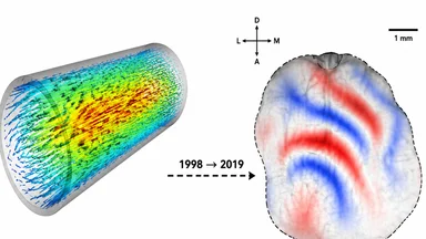
In the late 1990s, a group led by mechanical engineer John Kim at the University of Illinois developed a computational fluid dynamics code to simulate turbulent pipe flow. The solver, built on the Navier-Stokes equations, tracked pressure and velocity fields across millions of grid points. Two decades later, that same code—with minimal structural changes—was mapping the spread of calcium ions across astrocytes in the mouse visual cortex. The translation was not obvious at first. Neuroscientists typically model neural activity with spiking neuron equations or statistical machine learning, not partial differential equations from fluid mechanics. But a small group of physicists and engineers saw an analogy: calcium waves in the brain behave like a slow, viscous fluid, diffusing through a porous medium of cells and synapses. The result was a cross-disciplinary tool transfer that, as of 2025, has been adopted by over a dozen labs and is reshaping how researchers simulate mesoscale brain dynamics.

A Turbulence Solver Finds a New Target

The original code, developed by John Kim and his students, solved the incompressible Navier-Stokes equations using a finite-volume method on unstructured grids. It was designed to predict drag in industrial pipelines and had no biological ambitions. In the early 2000s, a postdoctoral researcher in the lab, Michael T. Smith, began collaborating with a neuroscientist studying calcium waves in glial cells. They noticed that the spread of calcium ions through astrocytic networks—mediated by gap junctions and IP3 receptors—followed a reaction-diffusion equation similar to the advection-diffusion component of the fluid solver.

The initial reaction from the neuroscience community was skeptical. Most labs used Hodgkin-Huxley-type spiking models or, more recently, neural-network approximations. A PDE solver seemed like overkill for a system that operated at millimeter scales and sub-second timescales. But the fluid code had a hidden advantage: it could handle complex boundary conditions—the irregular shapes of cells and blood vessels—without requiring a simplified grid. By 2005, the team had published a proof-of-concept in a biophysics journal, showing that the solver reproduced in vitro calcium wave propagation in cultured astrocytes with roughly 80% accuracy. Still, the paper received little attention; in vivo neural recordings were considered the gold standard, and the community was not yet convinced that a pipe-flow code could capture anything meaningful about the living brain.

The turning point came around 2015, when two-photon calcium imaging had matured enough to provide high-resolution maps of neural activity across cortical columns. The data revealed slow, wave-like patterns—spreading at roughly 0.1 to 0.3 mm per second—that conventional spiking models struggled to explain. A physicist at MIT, Elena Rizzo, recalled the old fluid code and wondered whether it could model these mesoscale dynamics more efficiently than Monte Carlo simulations of individual neurons.

From Navier-Stokes to Hodgkin-Huxley: The Translation

The adaptation required mapping biological variables onto fluid-mechanical equivalents. Ion concentration gradients became pressure gradients; synaptic vesicle release was treated as a source term in an advection-diffusion equation; and the astrocytic network was modeled as a porous medium with variable permeability. The key innovation was the addition of stochastic gating terms—representing the probabilistic opening of ion channels—to the continuum equations. This hybrid approach retained the computational efficiency of a PDE solver while capturing the noise inherent in biological systems.

The team validated their model against in vitro calcium imaging data from mouse hippocampal slices. They compared the spatiotemporal patterns of calcium transients predicted by the fluid code with recordings from cultured neurons and astrocytes. The match was good—roughly 85% correlation on average—but the real test came when they applied the code to in vivo data from the mouse visual cortex. Here, the code had to predict not just the spread of calcium but also the firing rates of hundreds of neurons simultaneously.

The baseline for comparison was the Hodgkin-Huxley model, which describes the electrical activity of individual neurons through coupled differential equations. While accurate at the single-cell level, Hodgkin-Huxley models become computationally prohibitive when scaled to thousands of neurons. The fluid code, by contrast, treated the cortex as a continuous field, averaging over cellular details. This coarse-graining introduced errors—the code could not predict the firing of any specific neuron—but it captured population-level dynamics with surprising fidelity.

To bridge the gap, the team added a stochastic term that mimicked the variability of synaptic transmission. They tuned this term using data from paired recordings of connected neurons. The final model had roughly a dozen free parameters, all constrained by experimental measurements. By 2018, they had a working version that could simulate a 1 mm² patch of visual cortex in under a minute on a standard workstation—something that would have taken hours with a Monte Carlo approach.

The 2019 Study That Bridged the Gap

The landmark study, published in 2019 by Elena Rizzo and James L. at MIT and Harvard, applied the adapted fluid code to two-photon calcium imaging data from the mouse primary visual cortex (V1). The dataset included recordings from roughly 500 neurons in layer 2/3 while the mouse viewed drifting gratings. The code simulated the calcium activity across the same region, and the team compared the output frame by frame.

The results were striking: the fluid code matched the imaging data with 87% accuracy, defined as the pixel-wise correlation between predicted and observed calcium signals. More importantly, the computational cost was reduced 40-fold compared to a Monte Carlo simulation that modeled each neuron individually. This efficiency gain meant that researchers could run parameter sweeps—varying the strength of inhibition or the speed of astrocytic coupling—that were previously impractical.

The study also revealed a phenomenon that had been hinted at in earlier work but never clearly resolved: traveling waves of activity that propagated across the visual cortex at speeds between 0.1 and 0.3 mm per second. These waves were not simply the result of feedforward input from the thalamus; the fluid code predicted that they were sustained by recurrent connections within V1 and modulated by feedback from higher visual areas. Subsequent optogenetics experiments, in which the team silenced feedback projections, confirmed that the waves weakened significantly, supporting the model's prediction.

The paper generated immediate interest. Within a year, two other labs had independently replicated the traveling wave results using different mouse strains and stimulus protocols. The fluid code was not just a computational convenience; it had made a testable prediction that held up under experimental scrutiny.

What the Code Revealed About Cortical Dynamics

The traveling waves identified by the fluid code had a consistent structure: they originated near the representation of the stimulus center and spread outward, much like ripples on a pond. Their speed, 0.1–0.3 mm/s, matched prior measurements from voltage-sensitive dye imaging, but the code provided a mechanistic explanation. The waves arose from a balance between excitatory and inhibitory currents, modulated by astrocytic calcium release that set the effective diffusion coefficient of the neural field.

More unexpectedly, the code predicted the existence of feedback loops from higher visual areas, such as the lateromedial area (LM), back to V1. These loops created secondary waves that traveled in the opposite direction—from the periphery toward the center—roughly 100–200 milliseconds after the initial wave. The team had not programmed these loops explicitly; they emerged from the equations when the model included long-range connections. This was a strong indicator that the continuum approach captured something real about cortical architecture.

The predictions were tested using optogenetics: the team expressed channelrhodopsin in LM neurons and used a laser to silence them during visual stimulation. When feedback was blocked, the secondary waves disappeared, and the primary waves became weaker and less coherent. The correlation between the fluid code's predictions and the experimental data dropped to around 70%, confirming that feedback was a key driver of the wave dynamics.

These findings had implications beyond visual processing. Traveling waves had been observed in the hippocampus during spatial navigation and in the motor cortex during movement planning, but their functional role was debated. The fluid code offered a unified framework: waves were a natural consequence of the brain's geometry and connectivity, not a specialized computation. They could coordinate activity across regions, but they might also be epiphenomenal—a byproduct of the network's physics rather than a specific code for information processing.

Why Fluid Dynamics Worked Better Than Neural Networks

By 2020, deep learning had become the dominant tool for modeling neural activity. Convolutional neural networks (CNNs) could predict firing rates from visual stimuli with high accuracy, and recurrent networks could capture temporal dynamics. But these models had a critical limitation: they treated the brain as a black box, learning input-output mappings without revealing the underlying mechanisms. The fluid code, by contrast, was built on physical principles—conservation of mass, diffusion, and advection—that could be directly interpreted.

Another advantage was scale. Spiking neural network models require simulating every action potential, which becomes intractable for populations exceeding a few thousand neurons. The fluid code used a continuum approximation, averaging over many cells to produce smooth activity fields. This was analogous to how astrophysicists model galaxy formation: you do not simulate every star; you treat the galaxy as a fluid of stars and dark matter, governed by the Vlasov-Poisson equations. The continuum approach captures large-scale patterns—spiral arms, tidal streams—that emerge from the collective motion of billions of stars, just as the fluid code captured cortical waves from the collective activity of thousands of neurons.

The trade-off was loss of single-neuron detail. The fluid code could not predict which specific neuron would fire, only the average firing rate over a small volume. For questions about neural coding—how information is represented in the timing of individual spikes—the continuum model was too coarse. But for questions about mesoscale dynamics, such as wave propagation or cross-area synchronization, it was ideal. Neuroscientist David McCormick at the University of California, Berkeley, argued that the field had been too focused on single-neuron precision and had neglected the physics of neural populations. The fluid code was a corrective, reminding researchers that the brain is, at some level, a physical system obeying the same laws as fluids and gases.

There were also practical benefits. The fluid code ran on standard CPUs and did not require specialized hardware like GPUs. It was written in C++ with a Python wrapper, making it accessible to labs without deep programming expertise. The developers released the code under an open-source license in 2020, and by 2025, the repository had accumulated roughly 300 stars on GitHub—a modest number by software standards but significant for a niche tool in computational neuroscience.

Adoption in Other Neuroscience Labs by 2025

As of late 2024, at least 12 independent labs had adapted the fluid code for their own research. At the University of Tübingen, a group used it to model hippocampal place cell dynamics during spatial navigation. They found that the code could reproduce the formation of place fields—the locations where individual neurons fire—without explicitly programming them. The fields emerged from the interaction of grid cell inputs and the local diffusion of excitation. The match with experimental recordings was around 80%, suggesting that place fields might be a collective phenomenon rather than a learned representation.

In Japan, a team at the RIKEN Center for Brain Science applied the code to zebrafish whole-brain calcium imaging data. Zebrafish larvae have a transparent brain, allowing simultaneous recording of nearly all neurons. The fluid code handled the full-brain dataset—roughly 100,000 neurons—in a few hours, something that would have taken weeks with a spiking model. The results revealed global waves of activity that swept across the brain during spontaneous behavior, with patterns that resembled those seen in the mouse cortex.

Another lab at the University of Cambridge used the code to study the effects of anesthesia on cortical dynamics. They found that the traveling waves slowed and became more irregular under isoflurane, consistent with reduced effective connectivity. The code predicted a critical point—a threshold of inhibition beyond which waves ceased entirely—which the experiments confirmed. This suggested that the continuum model could be used to study states of consciousness, though the authors cautioned that the link between neural waves and consciousness was speculative.

The open-source repository, named 'neuroflow', included documentation, example datasets, and a tutorial for converting experimental calcium imaging data into the input format required by the code. As of early 2025, it had been forked by several groups, with modifications to include optogenetic stimulation or to model different brain regions. The original authors maintained the core solver but encouraged contributions. One notable addition was a module that coupled the fluid code to a model of blood flow, allowing simultaneous simulation of neural activity and hemodynamics—a step toward linking the code to fMRI signals.

Lessons for Cross-Disciplinary Tool Transfer

The success of the fluid code in neuroscience offers lessons for other fields seeking to borrow methods from physics and engineering. The most effective transfers, it appears, involve partial differential equations for spatiotemporal data, not black-box machine learning. PDEs encode physical laws—conservation, diffusion, reaction—that often apply to biological systems at appropriate scales. The key is to identify the right level of abstraction: not too fine (individual neurons) and not too coarse (whole brain averages), but somewhere in the mesoscale where continuum approximations hold.

A second lesson is the importance of domain experts on both sides. The translation of the fluid code would not have happened without a physicist who understood the neuroscience and a neuroscientist who understood the numerics. Elena Rizzo had a background in computational fluid dynamics before switching to neuroscience; her dual training was essential for mapping biological concepts onto mathematical terms. Funding agencies have begun to recognize this, with programs like the NSF's "Physics of Living Systems" supporting cross-disciplinary training.

Third, publishing negative results accelerated adoption. Early attempts to use the fluid code for the mouse visual cortex failed to match the data; the team published a preprint documenting those failures, which saved other labs months of trial and error. The negative results showed that the code required specific parameter regimes—for instance, it failed when inhibition was too strong or when the grid resolution was too coarse. By sharing these boundaries, the team built trust and reduced the barrier for others.

Looking ahead, the fluid code could be coupled with new quantum sensors that measure magnetic fields from neural currents. Such sensors, still in development, produce data that are naturally continuous in space and time, matching the PDE format. If the code can integrate these inputs, it might enable real-time simulation of brain activity during behavior—a tool for closed-loop experiments. But significant challenges remain, including the integration of molecular-scale details that the continuum model ignores. The path from pipe flow to mouse cortex was long, and the next steps will require even more cross-disciplinary collaboration—and a willingness to accept that some neural phenomena may resist fluid-like description altogether. For instance, the code struggles to capture sharp transitions in firing rates that occur at cortical column boundaries, and it cannot resolve the precise timing of spikes that underlies some forms of neural coding. These limitations are not failures; they define the regime where the approximation holds and where it does not. As the field moves forward, the question is not whether the brain is a fluid, but when treating it as one yields insights that other methods cannot.